Polarimetric Decomposition Operator
This operator performs the following polarimetric
decompositions for a full polarimetric SAR product:
- Sinclair Decomposition
- Pauli Decomposition
- Freeman-Durden Decomposition
- Yamaguchi Decomposition
- H-a Alpha Decomposition
- Touzi Decomposition
- Van Zyl Decomposition
- Cloude Decomposition
- Generalized Freeman-Durden Decomposition
- Model-Free 3-Component Decomposition (MF3CF)
- Model-Free 4-Component Decomposition (MF4CF)
Sinclair Decomposition
Let
be the complex scatter matrix. The Sinclair
decomposition produces (R, G, B) bands with the following
intensities
- Red:
|Svv|2,
- Green:
|(Shv + Svh)/2|2,
- Blue:
|Shh|2,
The main drawback of this decomposition is the
physical interpretation of the resulting RGB image.
Pauli Decomposition
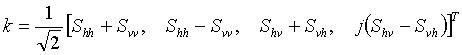
The (R, G, B) bands produced by the Pauli
decomposition correspond to the following intensities [1]:
- Red: 0.5*|Shh -
Svv|2, which represents the contribution
of single- or odd-bounce scattering to the final measured
scattering matrix
- Green: 0.5*|Shv +
Svh|2, which represents the scatter
power by targets that are able to return the orthogonal
polarization, for example the volume scattering produced by the
forest canopy
- Blue: 0.5*|Shh +
Svv|2, which represents the power
scattered by targets characterized by double- or
even-bounce
Freeman-Durden Decomposition
The Freeman decomposition models the covariance matrix
as the contribution of three scattering mechanisms [1]:
- canopy scatter from a cloud of randomly oriented dipoles,
forest for example;
- even- or double-bounce scatter from a pair of orthogonal
surfaces with different dielectric constants;
- Bragg scatter from a moderately rough surface.
The power scattered by the components of the
above three scattering mechanisms are employed to generate a RGB
image as the following:
- Red: the power scattered by
the double-bounce component of the covariance matrix
- Green: the power
scattered by the volume scattering component of the covariance
matrix
- Blue: the power
scattered by the surface-like scattering component of the
covariance matrix
Yamaguchi Decomposition
The three-component Freeman-Durden decomposition [1]
can be successfully applied to SAR observations under the
reflection symmetry assumption. However, there exists areas in an
SAR image where the reflection symmetry condition does not hold.
Yamaguchi et al. proposed, in 2005, a four-component scattering
model by introducing an additional term corresponding to
nonreflection symmetric cases. The fourth component introduced is
equivalent to a helix scattering power. This helix scattering power
term appears in heterogeneous areas (complicated shape targets or
man-made structures) whereas disappears for almost all natural
distributed scattering. Therefore, Yamaguchi decomposition models
the covariance matrix as the following four scattering mechanisms:
- volume;
- double-bounce;
- surface; and
- helix scatter components.
H-A-Alpha Decomposition
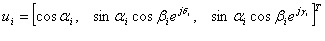
The H-A-Alpha decomposition [1] is based on the eigen
decomposition of the coherency matrix [T
3
]. Let
λ
1
,
λ
2
, and
λ
3
be the eigenvalues of the coherency matrix (
λ
1
>
λ
2
>
λ
3
> 0), and
u
1
,
u
2
and
u
3
be the corresponding eigenvectors which can be expressed as the
following:
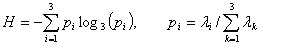
Then three secondary parameters are defined as the follows:
- Entropy:
- Anistropy:
- Alpha:
Touzi Decomposition
In 2007, for the monostatic scattering case, Ridha
Touzi has proposed in [2] a new Target Scattering Vector Model
(TSVM). Based on the Kennaugh-Huynen decomposition, this model
allows to extract four roll-invariant parameters:
- Kennaugh-Huynen maximum polarization parameter: orientation
angle (Ψ);
- Kennaugh-Huynen maximum polarization parameter: helicity (τ);
- Symmetric scattering type magnitude (α);
- Symmetric scattering type phase (Φ).
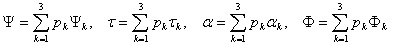
The roll-invariant incoherent target
decomposition, i.e. Touzi decomposition, is as the following:
- Compute target coherency matrix [T3] with a sliding
window;
- Perform eigendecomposition on the coherency matrix;
- Apply the new target scattering vector model to each
eigenvector to extract four parameters (Ψk,
τk,
αk,
Φk,
k = 1, 2, 3).
- Compute averaged parameters (Ψ,
τ,
α,
Φ):
Van Zyl Decomposition
The Van Zyl decomposition [1] assumes that the
reflection symmetry hypothesis establishes and the correlation
between co-polarized and cross-polarized channels is zero. The
assumption is generally true in case of natual media such as soil
and forest. With such an assumption, the eigen decomposition of the
averaged covariance matric C
3
can be given analytically and C
3
can be expressed in the following manner:
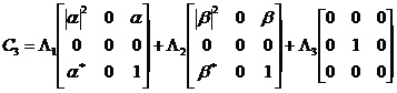
The van Zyl decomposition thus shows that the first two
eigenvectors represent equivalent scattering matrices that can be
interpreted in terms of odd and even numbers of reflections.
Cloude Decomposition
The Cloude decomposition [1] is an eigenvector based
decomposition. It idetifies the dominant scattering mechanism via
the extraction of the largest eigenvalue.
Generalized Freeman-Durden Decomposition
The Generalized Freeman-Durden decomposition in [3] is
also a model-based decomposition. Similar to the Freeman-Durden
decomposition, it assumes that the main backscattering
components are direct backscatter from the underlying surface,
double-bounce from a pair of orthogonal surfaces, and direct volume
scattering from the top layer. With the 2-layer model and the
assumptions above, we have more parameters than the measurements.
Generally, to invert the modle, more assumptions on the
parameters are needed.With the Generalized Freeman-Durden
decomposition, it is assumed that the surface and dihedral
mechanisms are orthogonal. Then the power scattered by the
three components can be computed by inverting the model.
Model-free 3 Component Decomposition (MF3CF)
Model-free 3 component decomposition technique [4]
does not consider any volume model for the computation of the three
scattering power components. The scattering power components are
roll-invariant. The total power is conserved after decomposition
and all the scattering power components are non-negative. The
target scattering type parameter is represented as:
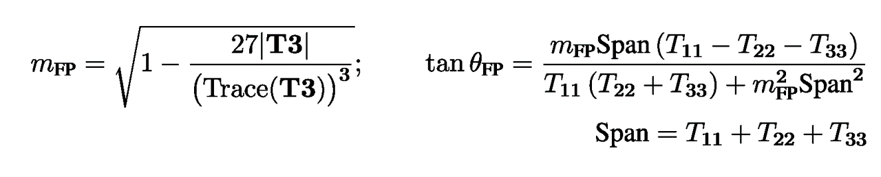
where, Θ
FP
is the target characterization parameter which varies from -45 to
45 degrees, m
FP
is the 3D Barakat degree of polarization, T
11
, T
22
and T
33
are the elements of the coherency matrix and Span is the total
power of coherency matrix T
3
.
The scattering power components are:
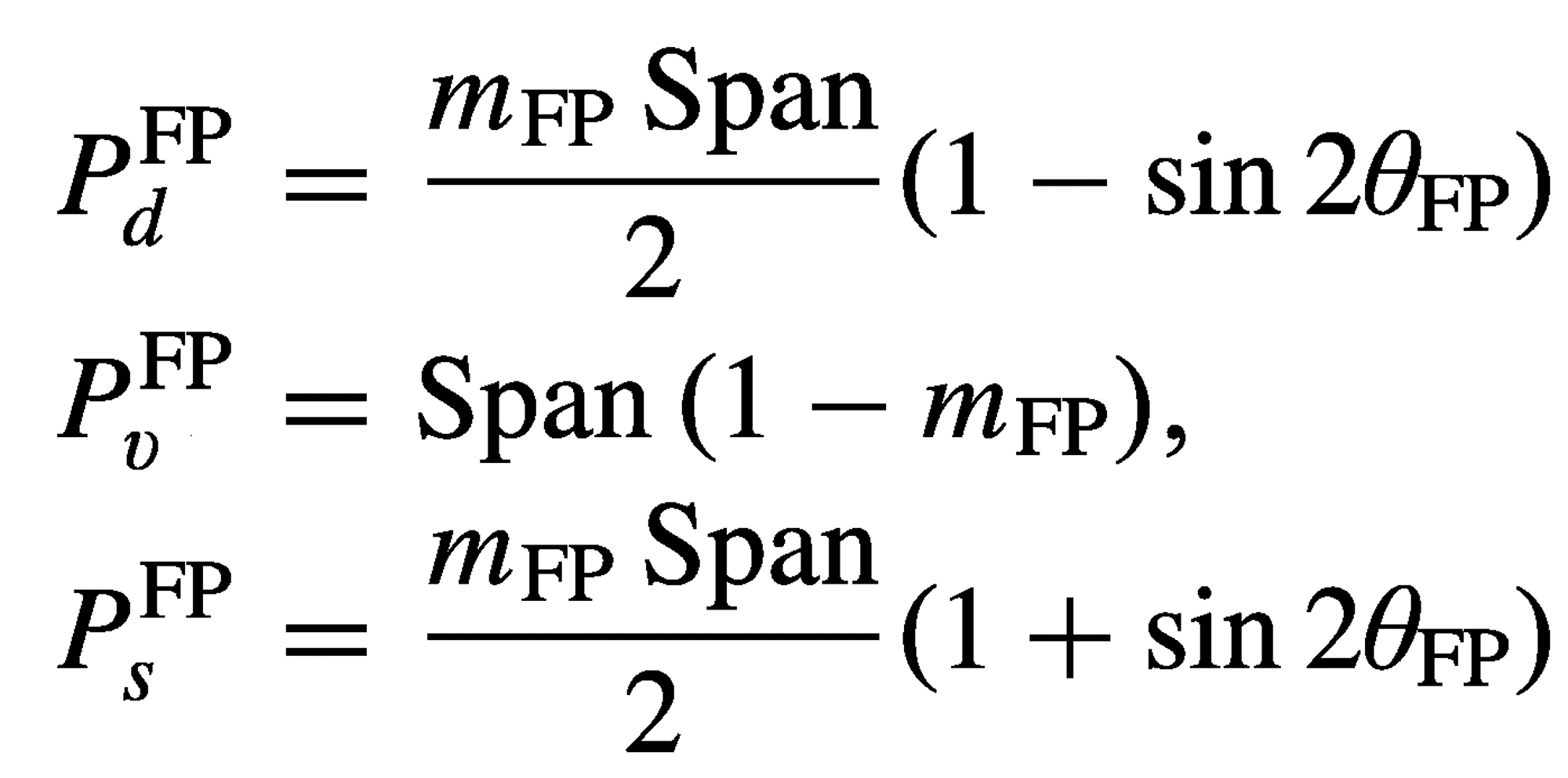
P
d
FP
is the even bounce power component, P
s
FP
is the odd bounce power component and P
v
FP
is the diffused power component.
Model-Free 4-Component Decomposition (MF4CF)
Model-free 4 component decomposition technique [5]
does not consider any volume model for the computation of the four
scattering power components. The scattering power components are
roll-invariant. The total power is conserved after decomposition
and all the scattering power components are non-negative. However,
in this decomposition a scattering asymmetry parameter is
introduced which captures the helicity.
The scattering type parameters are:
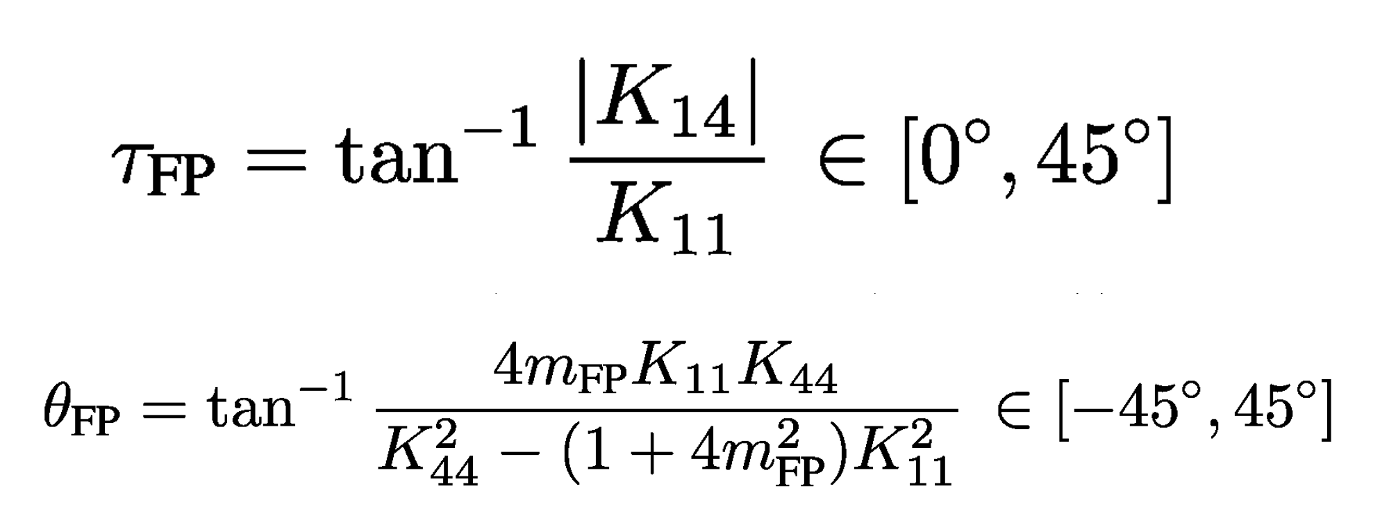
where, Τ
FP
is the target asymmetry parameter and Θ
FP
is the target characterization parameter. K
11
, K
14
and K
44
are the elements of the Kennaugh matrix.
The four scattering power components are:
P
d
is the even bounce power component, P
s
is the odd bounce power component, P
v
is the diffused power component and P
v
is the asymmetry (helix) power component.
Input and Output
- The input to this operator can be a full polarimetric SAR
product with 8 bands, i.e. I and Q bands for HH, VV, HV and VH
polarizations, or covariance matrix generated by Covariance Matrix
Generation operator, or coherency matrix output by Coherency Matrix
Generation operator.
- The output of this operator are bands corresponding to the
decomposition result.
Parameters Used
For all decompositions, the following processing
parameter is needed (see Figure 1):
- Decomposition: the decomposition method
Figure 1. Dialog box for Polarimetric
Decomposition operator
For Freeman-Durden decomposition, an extra parameter is needed (see
Figure 2):
- Window Size: dimension of sliding window for computing mean
covariance or coherence matrix
Figure 2. Dialog box for Freeman-Durden
decomposition
For Yamaguchi decomposition, the following parameters are needed
(see Figure 3):
- Window Size: dimension of sliding window for computing mean
covariance or coherence matrix
Figure 3. Dialog box for Yamaguchi
decomposition
For H-A-Alpha decomposition, the following extra parameters are
needed (see Figure 4):
- Window Size: dimension of sliding window for computing mean
covariance or coherence matrix
- Checkbox for outputing parameters Entropy (H), Anistropy (A)
and Alpha
- Checkbox for outputing parameters Beta, Delta, Gamma and
Lambda
- Checkbox for outputing parameters Alpha1, Alpha2 and
Alpha3
- Checkbox for outputing parameters Lambda1, Lambda2 and
Lambda3
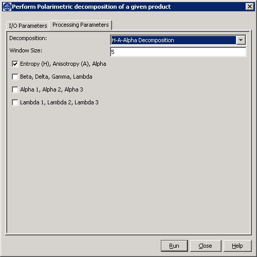
Figure 4. Dialog box for H-A-Alpha
decomposition
For Touzi decomposition, the following extra parameters are needed
(see Figure 5):
- Window Size: dimension of sliding window for computing mean
covariance or coherence matrix
- Checkbox for outputing parameters Psi, Tau, Alpha and Phi
- Checkbox for outputing parameters Psi1, Tau1, Alpha1 and
Phi1
- Checkbox for outputing parameters Psi2, Tau2, Alpha2 and
Phi2
- Checkbox for outputing parameters Psi3, Tau3, Alpha3 and
Phi3
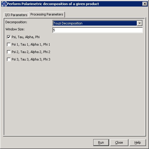
Figure 5. Dialog box for Touzi
decomposition
For Van Zyl decomposition, the following parameters are used (see
Figure 6):
- Window Size: dimension of sliding window for computing mean
covariance or coherence matrix
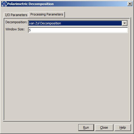
Figure 6. Dialog box for Van Zyl
decomposition
For Model-free 3 component decomposition (MF3CF) decomposition,
the following parameters are used (see Figure 7):
- Window Size: dimension of sliding window for computing mean
covariance or coherence matrix
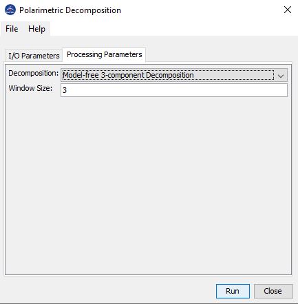
Figure 7. Dialog box for Model-free 3
component decomposition (MF3CF)
For Model-free 4 component decomposition (MF4CF) decomposition, the
following parameters are used (see Figure 8):
- Window Size: dimension of sliding window for computing mean
covariance or coherence matrix
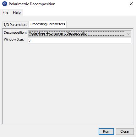
Figure 8. Dialog box for Model-free 4
component decomposition (MF4CF)
Reference:
[1] Jong-Sen Lee and Eric Pottier, Polarimetric Radar Imaging:
From Basics to Applications, CRC Press, 2009
[2] R. Touzi, “Target Scattering Decomposition in Terms of
Roll-Invariant Target Parameters,” IEEE Transactions on
Geoscience and Remote Sensing, vol. 45, no. 1, pp. 73–84,
January 2007.
[3] S.R. Cloude, “Polarisation: Applications in Remote
Sensing”, Oxford University Press, ISBN 978-0-19-956973-1,
2009.
[4] S. Dey, A. Bhattacharya, D. Ratha, D. Mandal and A. C.
Frery, 2020. “Target characterization and scattering power
decomposition for full and compact polarimetric SAR data”,
IEEE Transactions on Geoscience and Remote Sensing, 59(5),
pp.3981-3998.
[5] S. Dey, A. Bhattacharya, A. C. Frery, C.
López-Martínez and Y. S. Rao, 2021. “A
Model-free Four Component Scattering Power Decomposition for
Polarimetric SAR Data”, IEEE Journal of Selected Topics in
Applied Earth Observations and Remote Sensing, 14,
pp.3887-3902.