Orthorectification

SAR Simulation Terrain Correction Operator

The operator generates orthorectified image using rigorous SAR simulation.

Major Processing Steps

Some major steps of the procedure are listed below:

1. SAR simulation: Generate simulated SAR image using DEM, the geocoding and orbit state vectors from the original SAR image, and mathematical modeling of SAR imaging geometry. The simulated SAR image will have the same dimension and resolution as the original image. For detailed steps and parameters used in SAR simulation, please refer to the SAR Simulation Operator.
2. Co-registration: The simulated SAR image (reference) and the original SAR image (secondary) are co-registered and a WARP function is produced. The WARP function maps each pixel in the simulated SAR image to its corresponding position in the original SAR image. For detailed steps and parameters used in co-registration, please refer to the GCP Selection Operator.
3. Terrain correction: Traverse DEM grid that covers the imaging area. For each cell in the DEM grid, compute its corresponding pixel position in the simulated SAR image using SAR model. Then its corresponding pixel position in the original SAR image can be found with the help of the WARP function. Finally the pixel value for the orthorectified image can be obtained from the original SAR image using interpolation.

Products Supported

• ASAR (IMS, IMP, IMM, APP, APM, WSM), ERS products (SLC, IMP), RADARSAT-2, TerraSAR-X are fully supported.
• Some third party missions are not fully supported.

DEM Supported

Currently, only the DEMs with geographic coordinates (P_lat, P_lon, P_h) referred to global geodetic ellipsoid reference WGS84 (and height in meters) are properly supported.

Various different types of Digital Elevation models can be used (ACE, GETASSE30, ASTER, SRTM 3Sec GeoTiff).

The STRM v.4 (3” tiles) from the Joint Research Center FTP (xftp.jrc.it) will automatically be downloaded in tiles for  the area covered by the image to be orthorectified. The tiles will be downloaded to the folder .snap\AuxData\DEMs\SRTM_DEM\tiff.

Please note that for ACE and SRTM, the height information (being referred to geoid EGM96) is automatically corrected to obtain height relative to the WGS84 ellipsoid. For Aster Dem height correction is not yet applied.

Note also that the SRTM DEM covers area between -60 and 60 degrees latitude. Therefore, for orthorectification of product of high latitude area, different DEM should be used.

User can also use external DEM file in Geotiff format which, as specified above, must be with geographic coordinates (P_lat, P_lon, P_h) referred to global geodetic ellipsoid reference WGS84 (and height in meters).

Note that the same DEM is used by both SAR simulation and Terrain correction. The DEM is selected through SAR Simulation UI.

Pixel Spacing

Besides the default suggested pixel spacing computed with parameters in the metadata, user can specify output pixel spacing for the orthorectified image.

The pixel spacing can be entered in both meters and degrees. If the pixel spacing in one unit is entered, then  the pixel spacing in another unit is computed automatically.

The calculations of the pixel spacing in meters and in degrees are given by the following equations: 

pixelSpacingInDegree = pixelSpacingInMeter / EquatorialEarthRadius * 180 / PI;

pixelSpacingInMeter = pixelSpacingInDegree * PolarEarthRadius  * PI / 180;

where EquatorialEarthRadius = 6378137.0 m and PolarEarthRadius = 6356752.314245 m as given in WGS84. 

Radiometric Normalization

This option implements a radiometric normalization based on the approach proposed by Kellndorfer et al., TGRS, Sept. 1998 where

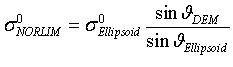
In current implementation θ_DEM is the local incidence angle projected into the range plane and defined as the angle between the incoming radiation vector and the projected surface normal vector into range plane[2]. The range plane is the plane formed by the satellite position, backscattering element position and the earth centre. 

Note that among σ^₀, γ^₀ and β^₀ bands output in the target product, only σ^₀ is real band while γ^₀ and β^₀ are virtual bands expressed in terms of σ^₀ and incidence angle. Therefore, σ^₀ and incidence angle are automatically saved and output if γ^₀ or β^₀ is selected.

For σ^₀ and γ^₀ calculation, by default the projected local incidence angle from DEM [2] (local incidence angle projected into range plane) option is selected, but the option of incidence angle from ellipsoid correction (incidence angle from tie points of the source product) is also available.

ENVISAT ASAR

The correction factors [3] applied to the original image depend on if the product is complex or detected and the selection of Auxiliary file (ASAR XCA file). 

Complex Product (IMS, APS)

• Latest AUX File (& use projected local incidence angle computed from DEM):

   The most recent ASAR XCA available from C:\Program Files\NEST4A\auxdata\envisat compatible with product date is automatically selected. According to this XCA file, calibration constant, range spreading loss and antenna pattern gain are obtained.

• • Applied factors:

  1. apply projected local incidence angle into the range plane correction

  2. apply calibration constant correction based on the XCA file
     

  3. apply range spreading loss correction based on the XCA file and DEM geometry
     

  4. apply antenna pattern gain correction based on the XCA file and DEM geometry
     

• External AUX File (& use projected local incidence angle computed from DEM):

   User can select a specific ASAR XCA file available from C:\Program Files\NEST4A\auxdata\envisat or from another repository. According to this selected XCA file, calibration constant, range spreading loss and antenna pattern gain are computed.

• • Applied factors:

  1. apply projected local incidence angle into the range plane correction

  2. apply calibration constant correction based on the selected XCA file
     

  3. apply range spreading loss correction based on the selected XCA file and DEM geometry
     

  4. apply antenna pattern gain correction based on the selected XCA file and DEM geometry
     

Detected Product (IMP, IMM, APP, APM, WSM)

• Latest AUX File (& use projected local incidence angle computed from DEM):

  The most recent ASAR XCA available from C:\Program Files\NEST4A\auxdata\envisat compatible with product date is automatically selected. Basically with this option all the correction factors applied to the original SAR image based on product XCA file used during the focusing, such as antenna pattern gain and range spreading loss, are removed first. Then new factors computed according to the new ASAR XCA file together with calibration constant and local incidence angle correction factors are applied during the radiometric normalisation process.

• • Applied factors:

  1. remove antenna pattern gain correction based on product XCA file

  2. remove range spreading loss correction based on product XCA file
     

  3. apply projected local incidence angle into the range plane correction
     

  4. apply calibration constant correction based on new XCA file

  5. apply range spreading loss correction based on new XCA file and DEM geometry

  6. apply new antenna pattern gain correction based on new XCA file and DEM geometry
     

• Product AUX File (& use projected local incidence angle computed from DEM):

   The product ASAR XCA file employed during the focusing is used. With this option the antenna pattern gain and range spreading loss are kept from the original product and only the calibration constant and local incidence angle correction factors are applied during the radiometric normalisation process.

• • Applied factors:

  1. apply projected local incidence angle into the range plane correction

  2. apply calibration constant correction based on product XCA file
     

• External AUX File (& use projected local incidence angle computed from DEM):

   User can select a specific ASAR XCA file available from the installation folder or from another repository. Basically with this option all the correction factors applied to the original SAR image based on product XCA file used during the focusing, such as antenna pattern gain and range spreading loss, are removed first. Then new factors computed according to the new selected ASAR XCA file together with calibration constant and local incidence angle correction factors are applied during the radiometric normalisation process.

• • Applied factors:

  1. remove antenna pattern gain correction based on product XCA file

  2. remove range spreading loss correction based on product XCA file
     

  3. apply projected local incidence angle into the range plane correction
     

  4. apply calibration constant correction based on new selected XCA file

  5. apply range spreading loss correction based on new selected XCA file and DEM geometry

  6. apply new antenna pattern gain correction based on new selected XCA file and DEM geometry
     

Please note that if the product has been previously multilooked then the radiometric normalization does not correct the antenna pattern and range spreading loss and only constant and incidence angle corrections are applied. This is because the original antenna pattern and the range spreading loss correction cannot be properly removed due to the pixel averaging by multilooking.

If user needs to apply a radiometric normalization, multilook and terrain correction to a product, then user graph “RemoveAntPat_Multilook_Orthorectify” could be used.

ERS 1&2

For ERS 1&2 the radiometric normalization cannot be applied directly to original ERS product.

Because of the Analogue to Digital Converter (ADC) power loss correction , a step before is required to properly handle the data. It is necessary to employ the Remove Antenna Pattern Operator which performs the following operations:

 For Single look complex (SLC, IMS) products

• apply ADC correction

For Ground range (PRI, IMP) products:

• remove antenna pattern gain
• remove range spreading loss
• apply ADC correction

After having applied the Remove Antenna Pattern Operator to ERS data, the radiometric normalisation can be performed during the Terrain Correction.

The applied factors in case of "USE projected angle from the DEM" selection are:

1. apply projected local incidence angle into the range plane correction
2. apply absolute calibration constant correction
3. apply range spreading loss correction based on product metadata and DEM geometry
4. apply new antenna pattern gain correction based on product metadata and DEM geometry

To apply radiometric normalization and terrain correction for ERS, user can also use one of the following user graphs:

• RemoveAntPat_Orthorectify
• RemoveAntPat_Multilook_Orthorectify

RADARSAT-2

• In case of "USE projected angle from the DEM" selection, the radiometric normalisation is performed applying the product LUTs and multiplying by (sin DEM/sin el), where DEM is projected local incidence angle into the range plane and el is the incidence angle computed from the tie point grid respect to ellipsoid.
• In case of selection of "USE incidence angle from Ellipsoid", the radiometric normalisation is performed applying the product LUT.

These LUTs allow one to convert the digital numbers found in the output product to sigma-nought, beta-nought, or gamma-nought values (depending on which LUT is used).

TerraSAR-X

• In case of "USE projected angle from the DEM" selection, the radiometric normalisation is performed applying
  
  1. projected local incidence angle into the range plane correction
  2. absolute calibration constant correction
• In case of " USE incidence angle from Ellipsoid " selection, the radiometric normalisation is performed applying
  
  1. projected local incidence angle into the range plane correction
  2. absolute calibration constant correction

Cosmo-SkyMed

• In case of "USE projected angle from the DEM" selection, the radiometric normalisation is performed deriving σ_⁰Ellipsoid [7] and then multiplying by (sinθ_DEM / sinθ_el), where θ_DEM is the projected local incidence angle into the range plane and θ_el is the incidence angle computed from the tie point grid respect to ellipsoid.
• In case of selection of "USE incidence angle from Ellipsoid", the radiometric normalisation is performed deriving σ_⁰Ellipsoid [7]
  

1. The local incidence angle is defined as the angle between the normal vector of the backscattering element (i.e. vector perpendicular to the ground surface) and the incoming radiation vector (i.e. vector formed by the satellite position and the backscattering element position) [2].
2. The projected local incidence angle from DEM is defined as the angle between the incoming radiation vector (as defined above) and the projected surface normal vector into range plane. Here range plane is the plane formed by the satellite position, backscattering element position and the earth centre [2].
   

Layover-Shadow Mask Generation

This operator can also generate layover-shadow mask for the orthorectified image. The layover effect is caused by the fact that the signal backscattered from the top of the mountain is actually received earlier than the signal from the bottom, i.e. the fore slope is reversed. The shadow effect is caused by the fact that no information is received from the back slope.  This operator generates the layover-shadow mask as a separate band using the 2-pass algorithm given in section 7.4 in [2]. The value coding for the layover-shadow mask is defined as the follows:

• 0 - corresponding image pixel is not in layover, nor shadow 
• 1 - corresponding image pixel is in layover
• 2 - corresponding image pixel is in shadow 
• 3 - corresponding image pixel is in layover and shadow

User can select output the layover-shadow mask by checkmarking "Save Layover-Shadow Mask as band" box in SAR-Simulation tab.

To visualize the layover-shadow mask, user can bring up the orthorectified image first, then go to layer manager and add the layover-shadow mask band as a layer.

Parameters Used

1. RMS Threshold: The criterion for eliminating invalid GCPs. (see Help for Warp Operator for detail)
2. WARP Polynomial Order: The degree of the WARP polynomial. The valid values are 1, 2 and 3. (see Help for Warp Operator for detail)
3. DEM Resampling Method: Interpolation method for obtaining elevation values from the original DEM file. The following interpolation methods are available: nearest neighbour, bi-linear, cubic convolution, bi-sinc and bi-cubic interpolations.
4. Image Resampling Method: Interpolation methods for obtaining pixel values from the source image. Three interpolation methods are available: nearest neighbour, bi-linear, cubic and bi-sinc interpolations.
5. Pixel Spacing (m): User can specify pixel spacing in meters for orthorectified image. If no pixel spacing is specified, then default pixel spacing computed from the source SAR image is used. For details, the reader is referred to Pixel Spacing section above.
6. Pixel Spacing (deg): User can also specify the pixel spacing in degrees.  If the value of any of the two pixel spacing is changed, the other one is updated automatically. For details, the reader is referred to Pixel Spacing section above.
7. Save DEM as band: Checkbox indicating that DEM will be save as a band in the target product.
8. Save local incidence angle as band: Checkbox indicating that local incidence angle will be save as a band in the target product.
9. Save projected local incidence angle as band: Checkbox indicating that the projected local incidence angle will be save as a band in the target product.
10. Save selected source band: Checkbox indicating that orthorectified images of user selected bands will be saved without applying radiometric normalization.
11. Apply radiometric normalization: Checkbox indicating that radiometric normalization will be applied to the orthorectified image.
12. Save Sigma0 as a band: Checkbox indicating that sigma0 will be saved as a band in the target product. The Sigma0 can be generated using projected local incidence angle, local incidence angle or incidence angle from ellipsoid.
13. Save Gamma0 as a band: Checkbox indicating that Gamma0 will be saved as a band in the target product. The Gamma0 can be generated using projected local incidence angle, local incidence angle or incidence angle from ellipsoid.
14. Save Beta0 as a band: Checkbox indicating that Beta0 will be saved as a band in the target product.
15. Auxiliary File: available only for ASAR. User selected ASAR XCA file for radiometric normalization. The following options are available: Latest Auxiliary File, Product Auxiliary File (for detected product only) and External Auxiliary File. By default, the Latest Auxiliary File is used. Details about the corrections applied according to the XCA selection are provided in Radiometric Normalisation – Envisat ASAR section above.
16. Show Range and Azimuth Shifts: Checkbox indicating that range and azimuth shifts (in m) for all valid GCPs will be displayed. The row and column shifts of each secondary GCP away from its initial position are output to a text file.

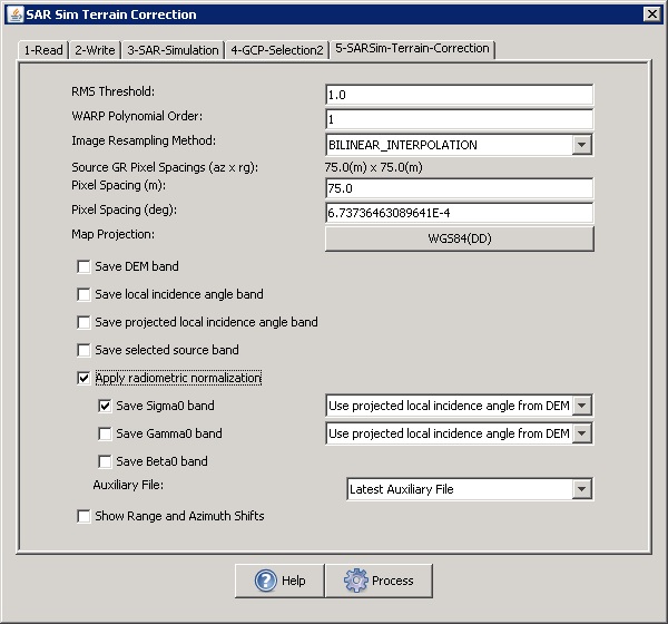
 Figure 1. SAR Sim Terrain Correction dialog box

Detailed Algorithm for Layover-Shadow Mask Generation

1. First a DEM image is created by the SAR Simulation operator using the geocoding of the original SAR image. The DEM image has the same dimension as the original SAR image with each pixel value of the DEM image is the elevation of the corresponding pixel in the original SAR image. 
2. Then 2-pass method (see section 7.4 in [2]) is applied to each range line in the DEM image to generate the layover and shadow mask for the DEM image. The 2-pass method compares the slant range for a DEM cell to slant ranges of other cells in the same range line to determine if the DEM cell will be imaged in layover or shadow area.
3. Next the layover-shadow mask for the DEM image is mapped to the simulated image to create the mask for the simulated image. The map is done using SAR simulation.
4. The layover-shadow mask for the simulated SAR image is then mapped to the original SAR image using the WARP function, which was created during co-registration of the simulated SAR image and the original SAR image.
5. Finally the mask for the original SAR image is mapped to the orthorectified image domain to produce the mask for the orthorectified image.

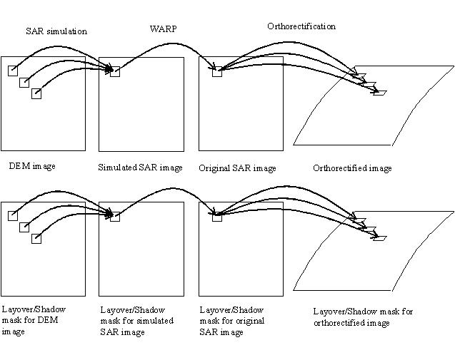
 Figure 2. Layover-shadow mask generation

Reference:

[1] Small D., Schubert A., Guide to ASAR Geocoding, RSL-ASAR-GC-AD, Issue 1.0, March 2008

[2] Schreier G., SAR geocoding: data and systems, Wichmann-Verlag, Karlsruhe, Germany, 1993

[3] Rosich B., Meadows P., Absolute calibration of ASAR Level 1 products, ESA/ESRIN, ENVI-CLVL-EOPG-TN-03-0010, Issue 1, Rev. 5, October 2004

[4] Laur H., Bally P., Meadows P., S�nchez J., Sch�ttler B., Lopinto E. & Esteban D., ERS SAR Calibration: Derivation of σ0 in ESA ERS SAR PRI Products, ESA/ESRIN, ES-TN-RS-PM-HL09, Issue 2, Rev. 5f, November 2004 

[5] RADARSAT-2 PRODUCT FORMAT DEFINITION - RN-RP-51-2713 Issue 1/7: March 14, 2008

[6] Radiometric Calibration of TerraSAR-X data - TSXX-ITD-TN-0049-radiometric_calculations_I1.00.doc, 2008

[7] For further details about Cosmo-SkyMed calibration please contact Cosmo-SkyMed Help Desk at info.cosmo@e-geos.it