
1. Software Installation and User’s Manual (SUM)
1.1. Introduction
This document is the Software Installation and User Manual (SUM) for the Sentinel-2 level 3 Processor for spatio temporal synthesis, labelled as Sen2Three.
Changes of release 1.1: Compatibility with PSD version 14.2 and Sentinel 2B products
- Sen2Three supports now the “safe compact” format which was introduced with PSD version 14.2 in parallel to the safe standard format as it was used up to PSD version 13.1. Sen2Three will detect the format automatically when reading a product. No configuration changes are necessary. The Level 3 output will always be generated in the PSD version 14.2 compatible safe compact format.
- If Sen2Three is detecting a version 13.1 formatted Level 2a input product, it will convert it first into a version 14.2 compatible safe compact Level 3 product and processes it afterwards. This allows a mixed input of Version 13.1 and 14.2 Level 2a products in the same directory at the same time.
- Sen2Three now also supports the processing of Sentinel 2B Level 2a input products and is compatible to Sen2Cor Version 2.4.0.
1.1.1. Purpose and Scope
This document is produced in the context of the development of the Sentinel 2 level 3 processor. Its purpose is to detail the Operation, Installation and Configuration of the Processor Software.
1.1.2. Applicable Documents
Table 1-1: Applicable Documents
| Reference | Code | Title | Issue |
|---|---|---|---|
| L3_ATBD | ATBD | Level 3 ATBD | 1.0 |
1.1.3. Reference Documents
Table 1-2: Reference Documents
| Reference | Code | Title | Issue |
|---|---|---|---|
| L3_DPMD | DPMD | Detailed Processing Model Documentation | 1.0 |
| L3_PFS | PFS | Product Format Specification | 1.1 |
| L3_IODD | IODD | Input Output Data Definition | 1.1 |
1.1.4. Acronyms and Abbreviations
All acronyms and abbreviations are listed in [L3-GLODEF]
1.1.5. Document Structure
This is the first part of a set of four documents describing the Sentinel 2 level 3 Processor for Spatio- Temporal synthesis, consisting of:
- Software Installation and User’s Manual (SUM), this document;
- Detailed Processing Model Documentation (DPMD);
- Product Format Specification (PFS);
- Input Output Data Definition (IODD).
Chapter 1.2, the Operational Concept describes the general usage of the processor, its algorithms and shows characteristic examples for the processing of the different algorithms.
Chapter 1.3, Installation and Setup describes in detail how the processor itself and its runtime environment will be installed and set up for operation.
Chapter 1.4, Configuration details the individual configuration parameters of the processor’s ground image processing parameters (GIPP).
Chapter 1.5, Operation describes how the processor will be operated from command line and as plugin inside of the SNAP toolbox.
Chapter 1.6, the Appendix will list among others the complete GIPP for reference.
1.2. Operational Concept
Sen2Three is a level 3 processor for the Spatio-Temporal Synthesis of bottom of atmosphere corrected level 2a images, as they are generated by the Sen2Cor application. Sen2Three takes time series of level 2a images of certain geographical areas as input and generates a synthetic output image by replacing step by step all invalid pixels of previous input images with the collocated valid pixels of scenes following in time.
Valid Pixels are hereby defined as primarily clear sky images with output pixels identified as vegetation (green), soils (yellow), or water (blue). Invalid Pixels are defined as medium and high probability clouds (medium grey and white), dark features or terrain shadows (dark grey), cloud shadows (brown) and optionally, thin cirrus (light blue) or snow (pink).
Scene Classification and the Radiometric Quality are obtained from the Sen2Cor level 2a algorithms for Atmospheric Correction, which is a necessary tool for obtaining the appropriate level 2a input products.
The level 3 spatio temporal synthesis algorithm generates a synthetic output image of a certain geographical area, divided into a series of “tiles”, using time series of collocated input images of the area and replacing step by step all contaminated (bad) pixels of the output with equivalent valid pixels. Input images are a collection of level 2a products acquired sequentially during a certain time period and prepared by Sen2Cor for subsequend processing. Figure 1.1 shows an overview on the general sequential processing chain.
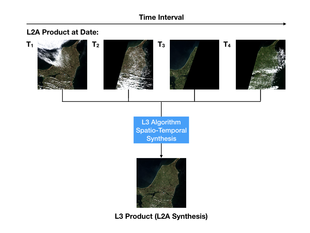
Fig. 1.1 Sequential Processing Chain
As the level 3 processing requires a full classification of the input scenes in order to perform its different synthesis algorithms, the scene classification algorithm of the Sen2Cor processor as a pre-processing step is always required. For level 2a input products this is performed during the level 2a processing via Sen2Cor. Non atmospheric corrected level 1c images can also serve as inputs. This is provided via an option of the Sen2Cor processor, where only a resampling of the L1c input products, followed by a scene classification is performed. See the Sen2Cor User Manual (L2A_SUM) for the special option ‘–sc_only”.
The Sen2Three algorithms work tile based. The spatio temporal synthesis will be performed separately for all tiles matching the same geographic area. If tiles are missing in some of the user products forming a data strip, these will be ignored.
During the pre-processing Sen2Three will generate a list of tiles to be processed. Only those tiles which match a certain time window will be accounted for the processing. The time window is configurable and can be specified in the Ground Image Processing Parameter (GIPP) File, which is located in the Sen2Three home directory (see Configuration).
1.2.1. Scene Classification
The Sen2Cor Scene Classification algorithm allows to detect clouds, snow and cloud shadows and to generate a classification map, which consists of 4 different classes for clouds (including cirrus), together with six different classifications for shadows, cloud shadows, vegetation, soils / deserts, water and snow. The algorithm is based on a series of threshold tests that use as input top-of-atmosphere reflectance from the Sentinel-2 spectral bands. In addition, thresholds are applied on band ratios and indexes like the Normalized Difference Vegetation - and Snow Index (NDVI, NDSI). For each of these thresholds tests, a level of confidence is associated. The algorithm uses the reflective properties of scene features to establish the presence or absence of clouds in a scene. Cloud screening is applied to the data in order to retrieve accurate atmospheric and surface parameters as used here for the level 3 processing. Figure 1.2 below shows the derivation of a scene classification from a level 1c input tile. The bar on the right shows the corresponding colour coding.
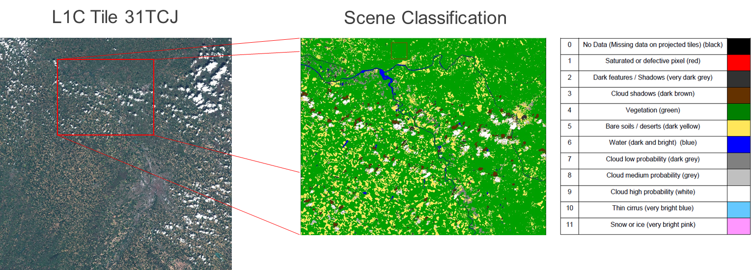
Fig. 1.2 Scene Classification
Table 1-3: Scene Classification Identifier
| Key | Value |
|---|---|
| NODATA | 0 |
| SATURATED_DEFECTIVE | 1 |
| DARK_FEATURES | 2 |
| CLOUD_SHADOW | 3 |
| VEGETATION | 4 |
| NOT_VEGETATED | 5 |
| WATER | 6 |
| UNCLASSIFIED | 7 |
| MEDIUM_PROBA_CLOUDS | 8 |
| HIGH_PROBA_CLOUDS | 9 |
| THIN_CIRRUS | 10 |
| SNOW_ICE | 11 |
1.2.2. Level 3 Synthesis
Valid pixels of a level 1c or level 2a input product are primarily clear sky areas in which the output pixels are identified to be of one of the three alternative pixel types vegetation (4), soils (5), or water (6). Invalid pixels are classified either as being clouds (7-9) or one of the pixel types 1-2. Cloud shadows (3), thin cirrus (10) and snow (11) can be optionally configured as belonging to the invalid pixel group.
The scene classification map introduced above will be updated during each sequential step. In an ideal synthesized scene only the five classes 4 - 6 and 11 (if permafrost occurs) would be present. However, as the Sen2Cor scene classificator has no ability to classify urban areas in the first run, those areas are initially classified as clouds of low or medium probability. As these areas are static, a small fraction of these two classes will remain, and thus (potentially) can be reclassified to urban areas in the long run.
1.2.3. Tile Map
A new level 3 map type will be generated and updated during the synthesis: the Tile Map is an indexed mosaic allowing conclusions on the history of the sequential synthesis. Each processed tile is indexed by a sequential number referring to the corresponding tile ID within the sequence. For the first three algorithms described in the following, the tile map thus gives an assignment between the output pixels and the tile they are origin. For the average algorithm, the meaning is different: here the sequential number marks how many tiles have been used for calculating the averaged single pixel values.
1.2.4. Algorithms
Four different algorithms are implemented, which determine the method how the final output product will be synthesized. For all images in all bands invalid pixels will always be replaced by good ones (if apparent). The replacement of pixels characterized as good will be performed according to following rules:
- Most Recent: good pixels of the output scene will always be replaced by good pixels of the current scene, if the time stamp of the recent scene is more actual that the time stamp of all past scenes.
- Temporal Homogeneity: good pixels of the output scene will be replaced by the equivalent good pixels of the current scene, if the sum of good pixels of the current scene is higher than the sum of good pixels of any scene in the past. This algorithm will always prioritize the “best” scenes in the course of time.
- Radiometric Quality: good pixels of the output scene will be replaced by by good pixels of the current scene, if either: the average of the Aerosol Optical Thickness is less or the average of the Solar Zenith Angle is higher than the equivalent parameter of the best scene in the past. The criteria are configurable. Again, this algorithm will always prioritize the “best” scenes in the course of time.
- Average: the output scene is an average of the good pixels of all processed scenes. The ‘Mosaic Map’ is the per pixel sum of all good pixels of the past scenes and is used for calculating the most recent average. In contrast to the former algorithms, the average will not prioritize a tile. Pixels of all tiles classified as valid will contribute to the final synthesized image.
If only cloudy pixels can be found for the previous scenes and the current sample, a prioritization based on lower cloud probability is performed.
Figure 1.3 and 1.4 below show the output of the Temporal Homogeneity algorithm: a tile map of indices is generated and updated during the synthesis: the colours of the tile map at top left represent those pixels obtained for the corresponding sequence. Figure 1.3 shows the synthesis at an early step, after three tiles have been accumulated. As none of the subsequent tiles 2 and 3 have a higher sum of valid pixels compared to tile 1, no update of the overall map is performed yet, and only invalid pixels are replaced. The gray bar in the upper histogram shows the frequency of pixels which have not been replaced at this stage, corresponding to the clouds as shown in the class map in the lower row.
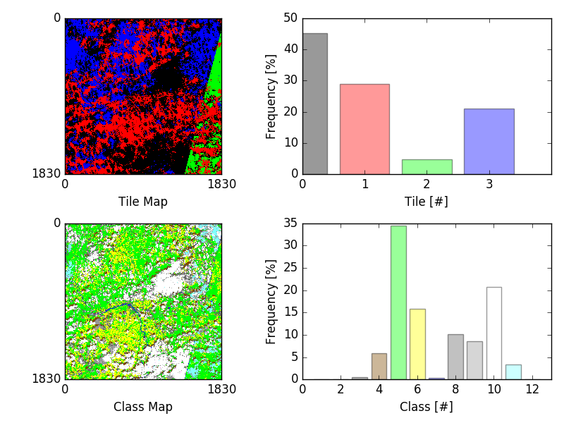
Fig. 1.3 Temporal Homogeneity Algorithm after 3 processing cycles.
The temporal homogeneity criterion influences the selection of valid pixels in order to get a final L3 synthesis rather composed with large patches of pixels acquired at the same date. This can be seen in a later stage of the same synthesis process: tile number 7 has the highest number of valid pixels and thus replaces all occurences of collocated valid pixels from the past. The sucessor, tile 8 in contrast has only a very limited contribution to the tile map.
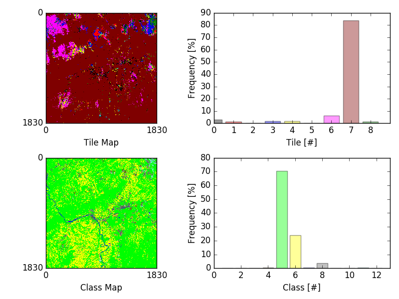
Fig. 1.4 Temporal Homogeneity Algorithm after 8 processing cycles.
In Figure 1.5 the average algorithm is used instead. Averaging can be useful in situations, when only a collection of very noisy input images are available in order to homogenize the output product. In this example, each pixel of the output product is an average between 1 and 6 valid pixels of all available input sequences. In contrast to the temporal homogeneity algorithm where the number (color) represents the according tile ID, the number in the tile map of Figure 1.5 represents the sum of tiles used for the averaging of the corresponding pixel. It is obvious that this kind of averaging will even out periodic changes in reflectance values, whereas the other algorithms might lead to strong contrasts between areas of different datatakes. It is in the responibility of the user to decide which algorithm is more appropriate for his specific needs.
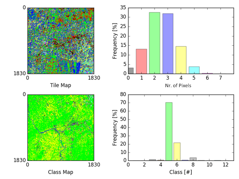
Fig. 1.5 Average Algorithm
Figure 1.6 shows a comparison between the outputs of the Temporal Homogeneity output vs. the Average algorithm. It can be seen that for the average output especially the soil pixels are somewhat brighter compared to the temporal homogeneity output, as it is the mean of several input images. The left tile shows the corresponding L2a best input tile.
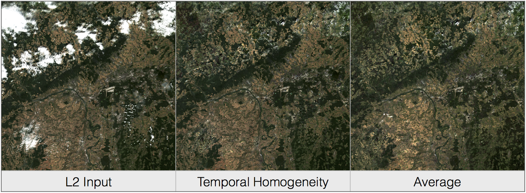
Fig. 1.6 Left: L2a Input, best scene, mid: Temporal Homogeneity, right: Average algorithm. Outputs after 8 iterations.
Figure 1.7 depicts a processing sequence of 8 consecutive tiles ordered by time. On the left the RGB composites of Bands 2-4 of the original level 2a input tiles, on the right, the synthesized tiles following the temporal homogeneity algorithm are shown.
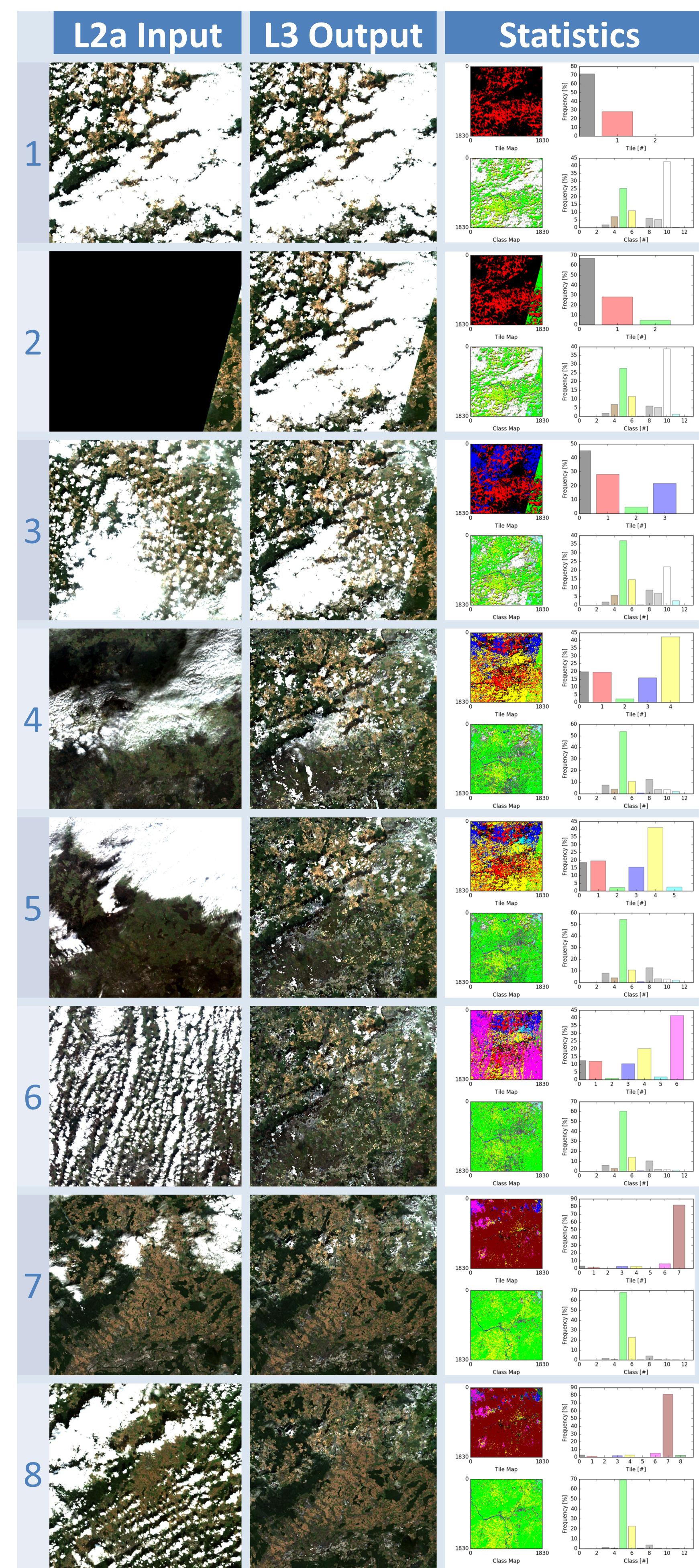
Fig. 1.7 Processing Sequence
1.2.5. Outputs
After the processing has been performed, a new level 3 user product will be generated and can be found in the Level 3 output directory as configured in the L3 GIPP configuration file (see below).
- New QI metadata for the level 3 synthesis, giving the statistics for the synthesized output product.
- The synthesized tile images for all bands for the given resolution.
- The updated scene classification excluding “invalid pixels” for all tiles.
- The L3 tile map for all tiles, showing the contingent of each individual input product to the final synthesized images as it is detailed in the statistics of the metadata.
All new metadata are described in detail in the Product Format Specification (PFS). The details on the generated products can be found in the Input Output Data Definition (IODD).
1.3. Installation and Setup
Sen2Three is completely written in Python 2.7. It will support the three following Operating Systems:
- Linux,
- Mac OSX,
- Windows,
(64 bit is mandatory).
The installation of the whole system is performed in two steps:
- Installation or upgrade of the Anaconda Runtime Environment
- Installation of the Processor itself.
The Sen2Three application works under the umbrella of the Anaconda (Python 2.7) distribution package. It is built using the Anaconda2 V.4.0 Development and Runtime Environment. A detailled description can be found here: (Anaconda2).
1.3.1. Anaconda Upgrade
If you have already installed Anaconda on you platform, due to an installation of Sen2Cor, no further action is necessary. If your Anaconda version should be updated, you can perform the following command via the command line:
C:\>conda update conda
Using Anaconda Cloud api site https://api.anaconda.org
Fetching package metadata: ....
Should end with displaying the following information:
conda                     4.0.5                    py27_0

C:\>conda update anaconda
Using Anaconda Cloud api site https://api.anaconda.org
Fetching package metadata: ....
Should end with displaying the following information:
anaconda 4.0.0 np110py27_0
Then, check the proper installation with:
C:\>python
Python 2.7.11 |Anaconda 4.0.0 (64-bit)| (default, Feb 16 2016, 09:58:36) [MSC v.1500 64 bit (AMD64)] on win32
Type "help", "copyright", "credits" or "license" for more information.
Anaconda is brought to you by Continuum Analytics.
Please check out: http://continuum.io/thanks and https://anaconda.org
You then can skip the next section and continue with the setup of Sen2Three.
1.3.2. Anaconda Installation from Scratch
If you never installed Anaconda before, then follow the steps below:
Download the recent version of the Anaconda python distribution for your operating system from: http://continuum.io/downloads and install it according to the default recommendations of the anaconda installer. It is strongly recommended to choose a local installation, except if you have the full administrator rights on your machine.
At the end of the installation, open a command line window and check the proper installation by typing “python.” It should display:
C:\>python
Python 2.7.11 |Anaconda 4.0.0 (64-bit)| (default, Feb 16 2016, 09:58:36) [MSC v.1500 64 bit (AMD64)] on win32
Type "help", "copyright", "credits" or "license" for more information.
Anaconda is brought to you by Continuum Analytics.
Please check out: http://continuum.io/thanks and https://anaconda.org
1.3.3. Deinstallation of an old Sen2Three installation
A deinstallation of an existing sen2three installation can be performed with:
C:\Users\<local_user>>pip uninstall sen2three
Uninstalling sen2three-1.0.0:
  c:\users\<local_user>\appdata\local\continuum\anaconda2\lib\site-packages\sen2three-1.0.1-py2.7.egg
  c:\users\<local_user>\appdata\local\continuum\anaconda2\scripts\l3_process-02.02.06-script.py
  c:\users\<local_user>\appdata\local\continuum\anaconda2\scripts\l3_process-02.02.06.exe
  c:\users\<local_user>\appdata\local\continuum\anaconda2\scripts\l3_process-1.0.1-script.py
  c:\users\<local_user>\appdata\local\continuum\anaconda2\scripts\l3_process-1.0.1.exe
  c:\users\<local_user>\appdata\local\continuum\anaconda2\scripts\l3_process-script.py
  c:\users\<local_user>\appdata\local\continuum\anaconda2\scripts\l3_process.exe

Proceed (y/n)? y
  Successfully uninstalled sen2three-1.0.1
If you have multiple Sen2Three versions installed, you can repeat the command until no further installations are found.
1.3.4. Sen2Three Installation
For Windows:
Download the zip archive from http://step.esa.int/main/third-party-plugins-2/sen2three and extract it with an unzip utility. Open a command line window and change the directory to the location where you have extracted the archive. Step into the folder sen2three-1.1.0, type:
python setup.py install
and follow the instructions. The setup will install the Sen2Three application and all its dependencies under the site-packages folder of the Anaconda python distribution. At the end of the installation you can select your home directory for the Sen2Three configuration data. This is by default:
”C:\Users\<your user account>\documents\sen2three”
The setup script generates the following two environment variables:
- SEN2THREE_HOME : this is the directory where the user configuration data are stored (see above). This can be changed later by you in setting the environment variable to a different location.
- SEN2THREE_BIN : this is a pointer to the installation of the Sen2Three package. This is located in the “site-packages” folder of Anaconda. Do not change this.
Open a new command line window, to be secure that your new environment settings are updated. From this new command line window perform the test below. This will give you a list of possible options:
C:\>L3_Process --help
usage: L3_Process.py [-h] [--resolution {10,20,60}] [--clean] directory

Sentinel-2 Level 3 Prototype Processor (SEN2THREE), 1.1.0, created:
2017.07.01, supporting Level-1C product version: 14.

positional arguments:
  directory             Directory where the Level-2A input files are located

optional arguments:
  -h, --help            show this help message and exit
  --resolution {10,20,60}
                        Target resolution, can be 10, 20 or 60m. If omitted,
                        all resolutions will be processed
  --clean               Removes the L3 product in the target directory before
                        processing. Be careful!

This will give you a list of possible further options how to operate.
If no errors are displayed, your installation was successful.
If no errors are displayed, your installation was successful.
For Linux and Mac:
Download the archive from http://step.esa.int/main/third-party-plugins-2/sen2three, and extract it with:
tar –xvzf sen2three-1.1.0.tar.gz
Open a shell, change the directory to the new created folder sen2three-1.1.0, type:
python setup.py install
and follow the instructions. The setup will install the Sen2Three application and all its dependencies under the site-packages folder of the Anaconda python distribution. At the end of the installation you can select your home directory for the Sen2Three configuration data. By default this is the directory where your $HOME environment variable points to. The setup script generates a script called “L3_Bashrc” and places it into the sen2three folder at your home directory. It contains the following two environment variables:
- SEN2THREE_HOME : this is the directory where the user configuration data are stored (see above). This can be changed later by you in setting the environment variable to a different location.
- SEN2THREE_BIN : this is a pointer to the installation of the Sen2Three package. This is located in the“site-packages” folder of the anaconda installation. Do not change this.
These settings are necessary for the execution of the processor. There are two possibilities how you can finish the setup:
- You can call this script automatically via your .bashrc or .profile script (OS dependent). For this purpose, add the line “source <location of your script>/L3_Bashrc” to your script.
- You can call this script also manually via “source L3_Bashrc” every time before starting the processor. However this is not recommended, as it may be forgotten.
Finally, to check the installation after sourcing the L3_Bashrc, call the processor via:
C:\>L3_Process --help
usage: L3_Process.py [-h] [--resolution {10,20,60}] [--clean] directory

Sentinel-2 Level 3 Prototype Processor (SEN2THREE), 1.1.0, created:
2017.07.01, supporting Level-1C product version: 14.

positional arguments:
  directory             Directory where the Level-2A input files are located

optional arguments:
  -h, --help            show this help message and exit
  --resolution {10,20,60}
                        Target resolution, can be 10, 20 or 60m. If omitted,
                        all resolutions will be processed
  --clean               Removes the L3 product in the target directory before
                        processing. Be careful!

This will give you a list of possible further options how to operate.
If no errors are displayed, your installation was successful.
1.4. Configuration
Configuration of the Sen2Three processor application is performed via an xml file which is called L3_GIPP. During installation this will be located in the cfg subdirectory of the Sen2Three home directory. This is is referenced by the environment variable $SEN2THREE_HOME (see above). The configuration parameters are listed in the following scheme. The configuration file is read in before the processing takes place and its parameters are validated for consistency according to the xsd scheme, which is fully listed in L3_GIPP.
1.4.1. L3_GIPP.xml
Table 1-4 shows the configuration of the Log_Level. The default is Info.
Table 1-4: Log level configuration
| Log_Level | |
|---|---|
|
|
| Key | Value |
| NOTSET | 0 |
| DEBUG | 1 |
| INFO | 2 |
| WARNING | 3 |
| ERROR | 4 |
| CRITICAL | 5 |
Table 1-5 summarizes two common configuration parameter.
If Display_Data is set to true, a graphic representation of the processing can be found in the QI_DATA subfolder of the GRANULE folder of a target product. This can be useful for controlling the operation of the different algorithms. The default setting is false.
By default, the level 3 target directory will be generated in the same folder where the L2a input products are located. The Target_Directory can be redirected to a different location by specifying an absolute path
Table 1-5: Common configuration parameter
| Key | Default | Type | Range | Description |
|---|---|---|---|---|
| Display_Data | false | string | n/a | Flag for graphical display of data. |
| Target_Directory | DEFAULT | string | n/a | Location of output data. |
Table 1-6 lists three filters for controlling which tiles should be processed. The Min_Time and Max_Time specify a time window which the acqired L1c / l2a user products must fulfill. Products with an acquisition date outside of this time window will be ignored. The Tile_Filter is either a list of tiles, separated by blanks or (*). If (*) is configured all tiles belonging to the input product will be processed. If a list of tiles (like ‘T32UMA T32UMB’) is assigned only those tiles will be processed.
Table 1-6: Level 3 synthesis
| Key | Default | Type | Range | Description | |
|---|---|---|---|---|---|
| Min_Time | n/a | time_str | n/a | Lower border acquisition time. | |
| Max_Time | n/a | time_str | n/a | Upper border acquisition time. | |
| Tile_Filter | n/a | str_list | n/a | A list of tiles separated by blanks. | |
Table 1-7 selects the Algorithm to be processed as described for Algorithms.
Table 1-7: Algorithm
| Algorithm | |
|---|---|
|
|
| Key | Type |
| MOST_RECENT | string |
| TEMP_HOMOGENEITY | string |
| RADIOMETRIC_QUALITY | string |
| AVERAGE | string |
Table 1-8 selects the preference if the RADIOMETRIC_QUALITY is selected as described for Algorithms.
Table 1-8: Radiometric preference
| Radiometric_Preference | |
|---|---|
|
|
| Key | Type |
| AEROSOL_OPTICAL_THICKNESS | string |
| SOLAR_ZENITH_ANGLE | string |
Table 1-9 lists the other additional options as can be used for fine tuning the algorithms:
Cirrus_Removal, Shadow_Removal and Snow_Removal can optionally be classified as invalid pixels. Default is true.
Max_Cloud_Probability and Max_Invalid_Pixels_Percentage can be configured as thresholds for terminating the algorithm. If one of the measured values falls below these treshold, the processing will terminate.
Max_Aerosol_Optical_Thickness and Max_Solar_Zenith_Angle are currently unused.
Median_Filter controls the smoothness of the invalid pixel mask. It the input data are contaminated of incoherent single invalid pixels an increase of the Median_Filter can possibly improve the results. It should not be higher than factor 3.
Table 1-9: Other options
| Key | Default | Type | Range | Description |
|---|---|---|---|---|
| Cirrus_Removal | true | bool | 0 : 1 | Activate cirrus removal. |
| Shadow_Removal | true | bool | 0 : 1 | Activate shadow removal. |
| Snow_Removal | true | bool | 0 : 1 | Activate snow removal. |
| Max_Cloud_Probability | n/a | ubyte | 0 : 100 | Terminate if reached. |
| Max_Invalid_Pixels_Percentage | n/a | ubyte | 0 : 100 | Terminate if reached. |
| Max_Aerosol_Optical_Thickness | n/a | ubyte | 0 : 100 | Currently unused. |
| Max_Solar_Zenith_Angle | n/a | ubyte | 0 : 70 | Currently unused. |
| Median_Filter | 1 | ubyte | 1:3 | Smoothing of area borders. |
A full specification of all configuration parameter can be obtained from L3_GIPP.
1.5. Operation
1.5.1. Command Line Tool
Sen2Three is a command line tool and works batch oriented. The full list of options can be retrieved by typing “L3_Process –help” via command line:
usage: L3_Process [-h] [--resolution {10,20,60}] [--clean] directory

Sentinel-2 Level 3 Prototype Processor (SEN2THREE), 1.1.0, created:
2015.09.15, supporting Level-1C product version: 13.

positional arguments:
  directory             Directory where the Level-2A input files are located

optional arguments:
  -h, --help            show this help message and exit
  --resolution {10,20,60}
                        Target resolution, must be 10, 20 or 60 [m]
  --clean               Removes all processed files in target directory. Be
                        careful!
The mandatory argument is the directory where the input files are located. The given path can either be absolute or relative. If a relative path is given, the processor expects to be called from the path where the input files are located. Otherwise it will show an error message, that the directory cannot be located. If an absolute path is given, it must point to the directory where the input product is located.
An optional argument is the resolution in which the processing shall take place. The Sen2Cor processor is able to generate three different resolutions (10, 20 or 60 m) which can be taken as input. If no resolution is specified, the processing will be performed for all three resolutions starting with the lowest one (60m).
Example:
sen2Three input_directory --resolution=20
Sen2Three processes all Level 2a products found in the input directory specified as positional argument. Following criteria are used for the processing:
- the input products must be complete Level 2a products as generated by Sen2Cor. The product root name must follow the following input mask: < S2?_????????????L2A_* > where a ‘?’ matches any single character and ‘*’ matches a sequence of any characters.
- Only those resolutions which are part of the input product will be taken into account.
- Only tiles with a time stamp between the ranges <Min_Time> and <Max_Time> configured in the L3_GIPP will be processed.
- If Tile_Filter in the L3_GIPP is ‘*’, all tiles will be processed. Else only the givel list of tiles will be processed. Example: T32UMA T32UMB ...
- The list of processed tiles can be found in the file called ‘processed’ in the L2a input directory. Those tiles will be ignored in a subsequent processing. This warrants that only new tiles or unprocessed resolutions will be processed when the processor is called again. Using this feature it is thinkable to start the Sen2Three processor in combination with Sen2Cor in form of a processing chain, where the data retrieval could be realized via the sentinels batch scripting API: https://scihub.copernicus.eu/userguide/5APIsAndBatchScripting
The option ‘–clean’ will remove the list of processed tiles and also the Level 3 target product so that the processing can be started from scratch.
1.5.2. Interfacing with the Sentinel 2 Toolbox
[TBD]
1.6. Appendix
1.6.1. Third Party Tools
Sen2Three was developed using the Anaconda2 V4.0 (Python 2.7) distribution. The following third party tools are already part of the Anaconda distribution, so that a separate installation is not neccesary, providing that Anaconda has been properly installed.
- MatPlotLib, for the graphical preparation of the output data;
- Objectify, elementTree for XML interfacing;
- numpy, scipy for statistics and image data handling;
- pytables for a faster interfacing with the image arrays.
The interface for reading and writing the JPEG 2000 image data was realized using a customized version of the OpenJPEG library (2.1.0) as provided by the Sentinel-2 Toolbox Development (s2tbx) and the glymur interface for accessing the OpenJPEG library via python.
For the development, runtime, debug and testing environment the excellent PyCharm IDE was used. This online documentation was realized with Sphinx, which is also part of the Anaconda distribution.
1.6.2. L3_GIPP
Contents of the level 3 Ground Image Processing Parameters:
<?xml version="1.0"  encoding="UTF-8"?>
<Level-03_Ground_Image_Processing_Parameter
  xmlns:xsi="http://www.w3.org/2001/XMLSchema-instance"
  xsi:noNamespaceSchemaLocation="L3_GIPP.xsd">
  <Common_Section>
    <Log_Level>INFO</Log_Level>
    <!-- NOTSET, DEBUG, INFO, WARNING, ERROR, CRITICAL -->
    <Display_Data>false</Display_Data>
    <Target_Directory>DEFAULT</Target_Directory>
    <PSD_Scheme PSD_Version="13" PSD_Reference="S2-PDGS-TAS-DI-PSD-V13.1_Schema">
        <UP_Scheme_2A>S2_User_Product_Level-2A_Metadata.xsd</UP_Scheme_2A>
        <UP_Scheme_3>S2_User_Product_Level-3_Metadata.xsd</UP_Scheme_3>
        <Tile_Scheme_2A>S2_PDI_Level-2A_Tile_Metadata.xsd</Tile_Scheme_2A>
        <Tile_Scheme_3>S2_PDI_Level-3_Tile_Metadata.xsd</Tile_Scheme_3>
        <DS_Scheme_2A>S2_PDI_Level-2A_Datastrip_Metadata.xsd</DS_Scheme_2A>
        <DS_Scheme_3>S2_PDI_Level-3_Datastrip_Metadata.xsd</DS_Scheme_3>
    </PSD_Scheme>
    <PSD_Scheme PSD_Version="14" PSD_Reference="S2-PDGS-TAS-DI-PSD-V14.2_Schema">
        <UP_Scheme_2A>S2_User_Product_Level-2A_Metadata.xsd</UP_Scheme_2A>
        <UP_Scheme_3>S2_User_Product_Level-3_Metadata.xsd</UP_Scheme_3>
        <Tile_Scheme_2A>S2_PDI_Level-2A_Tile_Metadata.xsd</Tile_Scheme_2A>
        <Tile_Scheme_3>S2_PDI_Level-3_Tile_Metadata.xsd</Tile_Scheme_3>
        <DS_Scheme_2A>S2_PDI_Level-2A_Datastrip_Metadata.xsd</DS_Scheme_2A>
        <DS_Scheme_3>S2_PDI_Level-3_Datastrip_Metadata.xsd</DS_Scheme_3>
    </PSD_Scheme>
    <GIPP_Scheme>L3_GIPP.xsd</GIPP_Scheme>
  </Common_Section>
  <L3_Synthesis>
    <Min_Time>2016-01-01T00:00:00Z</Min_Time>
    <Max_Time>2017-12-31T23:59:59Z</Max_Time>
    <Tile_Filter>*</Tile_Filter>
    <Algorithm>TEMP_HOMOGENEITY</Algorithm>
    <!-- MOST_RECENT, TEMP_HOMOGENEITY, RADIOMETRIC_QUALITY, AVERAGE -->
    <Radiometric_Preference>AEROSOL_OPTICAL_THICKNESS</Radiometric_Preference>
    <!-- AEROSOL_OPTICAL_THICKNESS, SOLAR_ZENITH_ANGLE -->
    <Cirrus_Removal>true</Cirrus_Removal>
    <Shadow_Removal>true</Shadow_Removal>
    <Snow_Removal>true</Snow_Removal>
    <Max_Cloud_Probability>0.0</Max_Cloud_Probability>
    <Max_Invalid_Pixels_Percentage>0.0</Max_Invalid_Pixels_Percentage>
    <Max_Aerosol_Optical_Thickness>0.0</Max_Aerosol_Optical_Thickness>
    <Max_Solar_Zenith_Angle>0.0</Max_Solar_Zenith_Angle>
    <Median_Filter>3</Median_Filter>
  </L3_Synthesis>
  <Classificators>
    <NO_DATA>0</NO_DATA>
    <SATURATED_DEFECTIVE>1</SATURATED_DEFECTIVE>
    <DARK_FEATURES>2</DARK_FEATURES>
    <CLOUD_SHADOWS>3</CLOUD_SHADOWS>
    <VEGETATION>4</VEGETATION>
    <NOT_VEGETATED>5</NOT_VEGETATED>
    <WATER>6</WATER>
    <UNCLASSIFIED>7</UNCLASSIFIED>
    <MEDIUM_PROBA_CLOUDS>8</MEDIUM_PROBA_CLOUDS>
    <HIGH_PROBA_CLOUDS>9</HIGH_PROBA_CLOUDS>
    <THIN_CIRRUS>10</THIN_CIRRUS>
    <SNOW_ICE>11</SNOW_ICE>
    <URBAN_AREAS>12</URBAN_AREAS>
  </Classificators>
</Level-03_Ground_Image_Processing_Parameter>
A full specification of all configuration parameter above can be obtained from L3_GIPP.